An Introduction to Virtual Adversarial Training
Divam Gupta
Virtual Adversarial Training is an effective regularization technique which has given good results in supervised learning, semi-supervised learning, and unsupervised clustering.
Get the source code used in this post from here
Virtual adversarial training has been used for:
- Improving supervised learning performance
- Semi-supervised learning
- Deep unsupervised clustering
There are several regularization techniques which prevent overfitting and help the model generalize better for unseen examples. Regularization helps the model parameters to be less dependent on the training data. The two most commonly used regularization techniques are Dropout and L1/L2 regularization.
In L1/L2 regularization, we add a loss term which tries to reduce the L1 norm or the L2 norm of the weights matrix. Small value of weights would result in simpler models which are less prone to overfitting.
In Dropout, we randomly ignore some neurons while training. This makes the network more robust to noise and variation in the input.
In neither of the two techniques mentioned, the input data distribution is taken into account.
Local distributional smoothness
Local distributional smoothness (LDS) can be defined as the smoothness of the output distribution of the model, with respect to the input. We do not want the model to be sensitive to small perturbations in the inputs. We can say that, there should not be large changes in the model output with respect to small changes in the model input.
In LDS regularization, smoothness of the model distribution is rewarded. It is also invariant of the parameters on the network and only depends on the model outputs. Having a smooth model distribution should help the model generalize better because the model would give similar outputs for unseen data-points which are close to data-points in the training set. Several studies show that making the model robust against small random perturbations is effective for regularization.
An easy way for LDS regularization is to generate artificial data-points by applying small random perturbations on real data points. After that encourage the model to have similar outputs for the real and perturbed data points. Domain knowledge can also be used to make better perturbations. For example, if the inputs are images, various image augmentation techniques such as flipping, rotating, transforming the color can be used.
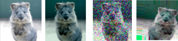 Example of input data transformation
Virtual adversarial training
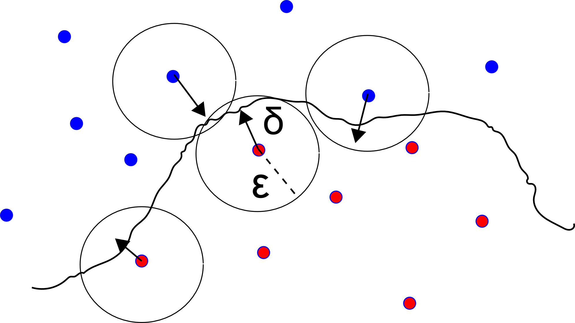
Virtual adversarial training is an effective technique for local distribution smoothness. Pairs of data points are taken which are very close in the input space, but are very far in the model output space. Then the model is trained to make their outputs close to each other. To do that, a given input is taken and perturbation is found for which the model gives very different output. Then the model is penalized for sensitivity with the perturbation.
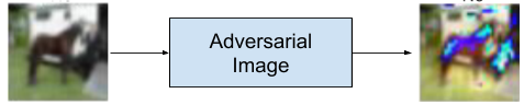 Step 1 : Generate the adversarial image
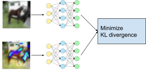 Step 2: Minimize the KL divergence
The key steps for virtual adversarial training are:
- Begin with an input data point x
- Transform x by adding a small perturbation r, hence the transformed data point will be T(x) = x + r
- The perturbation r should be in the adversarial direction – model output of the perturbed input T(x) should be different from the output of non-perturbed input. In particular, the KL divergence between the two output distributions should be maximum, while ensuring the L2 norm of r to be small. From all the perturbations r, let rv-adv be the perturbation in the adversarial direction.
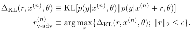
- After finding the adversarial perturbation and the transformed input, update the weights of the model such that the KL divergence is minimized. This would make the model robust towards different perturbations. The following loss is minimized via gradient descent:
During the virtual adversarial training, the model becomes more robust against different input perturbations. As the model becomes more robust, it becomes harder to generate perturbations and a drop in the loss is observed.
This method can be seen as similar to generative adversarial networks. But there are several differences:
- Rather than having a generator to fool the discriminator, a small perturbation is added to the input, in order to fool the model in thinking they are two vastly different inputs.
- Rather than discriminating between fake and real, the KL divergence between the model outputs is used. While training the model ( which is analogous to training the discriminator) we minimize the KL divergence.
Virtual adversarial training can be thought of as an effective data augmentation technique where we do not need prior domain knowledge. This can be applied to all kinds of input distributions, hence useful for true “unsupervised learning”.
How is virtual adversarial training different from adversarial training?
In adversarial training, labels are also used to generate the adversarial perturbations. The perturbation is generated such that classifier’s predicted label y’ becomes different from the actual label y.
In virtual adversarial training, no label information is used and the perturbation is generated using just the model outputs. The perturbation is generated such that output of the perturbed input is different from the model output of the original input ( as opposed to the ground truth label).
Implementing virtual adversarial training
Now we will implement basic virtual adversarial training using Tensorflow and Keras. The full code can be found here
First, define the neural network in Keras
network = Sequential()
network.add( Dense(100 ,activation='relu' ,  input_shape=(2,)))
network.add( Dense( 2  ))
Define the model_input , the logits p_logit by applying the input to the network and the probability scores p by applying softmax activation on the logits.
model_input = Input((2,))
p_logit = network( model_input )
p = Activation('softmax')( p_logit )
To generate the adversarial perturbation, start with random perturbation r and make it unit norm.
r = tf.random_normal(shape=tf.shape( model_input ))
r = make_unit_norm( r )
The output logits of the perturbed input would be p_logit_r
p_logit_r = network( model_input + 10*r )
Now compute the KL divergence of logits from the input and the perturbed input.
kl = tf.reduce_mean(compute_kld( p_logit , p_logit_r ))
To get the adversarial perturbation, we need an r such that the KL-divergence is maximized. Hence take the gradient of kl with respect to r. The adversarial perturbation would be the gradient. We use the stop_gradient function because we want to keep r_vadv fixed while back-propagation.
grad_kl = tf.gradients( kl , [r ])[0]
Finally, normalize the norm adversarial perturbation. We set the norm of r_vadv to a small value which is the distance we want to go along the adversarial direction.
r_vadv = make_unit_norm( r_vadv )/3.0
Now we have the adversarial perturbation r_vadv , for which the model gives a very large difference in outputs. We need to add a loss to the model which would penalize the model for having large KL-divergence with the outputs from the original inputs and the perturbed inputs.
p_logit_r_adv = network( model_input  + r_vadv )
vat_loss =  tf.reduce_mean(compute_kld( tf.stop_gradient(p_logit), p_logit_r_adv ))
Finally, build the model and attach the vat_loss .
model_vat = Model(model_input , p )
model_vat.add_loss( vat_loss   )
model_vat.compile( 'sgd' ,  'categorical_crossentropy'  ,  metrics=['accuracy'])
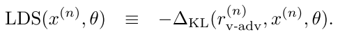
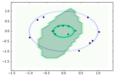
Now let’s use some synthetic data to train and test the model. This dataset is two dimensional and has two classes. Class 1 data-points lie in the outer ring and the class 2 data-points lie in the inner ring. We are using only 8 data-points per class for training, and 1000 data-points for testing.
 The plot of the synthetic dataset on a 2D plane
Let’s train the model by calling the fit function.
model.fit( X_train , Y_train_cat )
Visualizing model outputs
Now, let’s visualize the output space of the model along with training and the testing data.
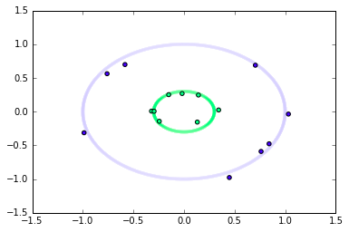
 Model decision boundary with virtual adversarial training
For this example dataset, it is pretty evident that the model with virtual adversarial training has generalized better and its decision boundary lies in the bounds of the test data as well.
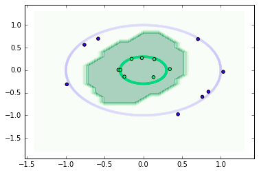
 Model decision boundary without virtual adversarial training
For the model without virtual adversarial training, we see some overfitting on the training data-points. The decision boundary, in this case, is not good and overlapping with the other class.
Applications of virtual adversarial training
Virtual adversarial training has shown incredible results for various applications in semi-supervised learning and unsupervised learning.
VAT for semi-supervised learning: Virtual adversarial training has shown good results in semi-supervised learning. Here, we have a large number of unlabeled data-points and a few labeled data points. Applying the vat_loss on the unlabeled set and the supervised loss on the labeled set gives a boost in testing accuracy. The authors show the superiority of the method over several other semi-supervised learning methods. You can read more in the paper here.
Virtual adversarial ladder networks: Ladder networks have shown promising results for semi-supervised classification. There, at each input layer, random noise is added and a decoder is trained to denoisify the outputs at each layer. In virtual adversarial ladder networks, rather than using random noise, adversarial noise is used. You can read more in the paper here.
Unsupervised clustering using self-augmented training: Here the goal is to cluster the data-points in a fixed number of clusters without using any labeled samples. Regularized Information Maximization is a technique for unsupervised clustering. Here the mutual information between the input and the model output is maximized. IMSAT has extended the approach by adding virtual adversarial training. Along with the mutual information loss, the authors apply the vat_loss. They show great improvements after adding virtual adversarial training. You can read more in the paper and my earlier blog post.
Conclusion
In this post, we discussed an efficient regularization technique called virtual adversarial training. We also dived in the implementation using Tensorflow and Keras. We observed that the model with VAT performs better when there are very few training samples. We also discussed various other works which use virtual adversarial training. If you have any questions or want to suggest any changes feel free to contact me or write a comment below.
Get the full source code from here
References
- Explaining and Harnessing Adversarial Examples
- Distributional Smoothing with Virtual Adversarial Training
- Virtual Adversarial Training: A Regularization Method for Supervised and Semi-Supervised Learning
- Virtual Adversarial Ladder Networks For Semi-supervised Learning
- Learning Discrete Representations via Information Maximizing Self-Augmented Training
